
So, if you haven't been able to tell from the sidebar already, I do a lot of stuff with fractals, for two reasons: first, they present a fun challenge to parallelize and can be incredibly satisfying to get working, and second, they make pretty pictures!
The second one was particularly important when I found the Wikipedia article on Buddhabrot one night about four years ago. I decided it looked so cool that I was gonna code it the very next day! A week later, I had a somewhat-working implementation written in Java (since it was the only language I knew at the time) using JOCL. It was fast, but the images it produced were downright garbage since I had zero knowledge of parallel programming other than "it made things faster".
Over this past winter break, I had a ton of time and nothing to do, so I decided to revive the project in C. I had just aced a parallel programming class, so I had the knowledge I lacked when I tried so long ago. I ended up pulling it off, learning a ton in the process.
Fractals 101
Fractals are just mathematically-generated images with infinite complexity. That is, no matter how far you zoom in, you'll always see more detail. The beautiful part of them is that they're usually extremely simple to describe. Jonathan Coulton even explained the Mandelbrot set in just a few lines of his eponymous song:
Just take a point called z in the complex plane,
Let z1 be z2+z,
z2 is z12+z,
z3 is z22+z, and so on
If the series of z(n) will always stay,
Close to z and never trend away,
That point is in the Mandelbrot set.
As you may have guessed from the name, the Buddhabrot set is very closely related to the Mandelbrot set. The only difference is that the Buddhabrot set records and plots every value of z on the image rather than simply using them to determine a point's membership in the set. This tiny tweak to the formula makes it more complicated to compute in parallel because it requires multiple threads to potentially access the same pixel's data simultaneously. The Mandelbrot set, on the other hand, computes each pixel independently of all other pixels, making that computation embarrasingly parallel and much easier to execute.
Racy Operations
Since Buddhabrot requires each thread to access and increment arbitrary "pixels" on the output, a race condition is sure to crop up if steps are not taken to mitigate it. If you check the "Unsafe Mode" box in Pbrot and use more than one thread, that's exactly what'll happen. The image is nearly identical to the default, race condition-free image because of the sheer resolution of the problem, but I saw an opportunity to investigate different methods to avoid it and decided to try them out.
I ran some tests using OpenMP's two built-in synchronization constructs, atomic and critical, as well as my own solution and the baseline. Pbrot only accesses the array in one line, so here it is with atomic:
#pragma omp atomic
	grid[coord]++;
And critical:
#pragma omp critical
{
	grid[coord]++;
}
The solution that I made up on my own and eventually used was simply to give each thread its own copy of the output grid, then combine them together at the end. This avoids the overhead of OpenMP's synchronization implementations, but requires far more memory. Its code is also a little more complex, but still not hard:
for (k = 0; k < numThreads; k++) {
	grid[k] = malloc(sizeof(OMPbucket_t) * gridSize * gridSize);
}

// ...

grid[threadNum][coord]++;
Now that we have our code, let's take a look at the results! 1
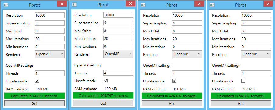
| Method | Time (s) | Time (relative) |
|---|---|---|
| Unsafe (race condition) | 44.887 | 1.000 |
| Atomic | 369.747 | 8.232 |
| Critical | 426.404 | 9.499 |
| Independent grids | 56.307 | 1.254 |
Right away, we can see that atomic operations and critical sections are much, much slower than our baseline. An 8x performance penalty is unacceptable. I don't know enough about the implementation of atomic operations or mutexes on x86 processors to take a guess as to why their performance is so bad, but these results reveal that they should be used sparingly whenever possible. The slight performance degradation in the independent grids approach is easily explained by caching; running this test with a smaller grid size but higher supersampling gives virtually identical results for the unsafe and independent grid runs. Assuming the system has enough RAM to fit all the extra copies of the grid, this approach is by far the best for avoiding race conditions.
Work Smarter, Not Harder
Buddhabrot requires calculating the z values of each point until we either reach the maximum allowed number of iterations, in which case we just move onto the next point and start over, or one z value gets too far away from c. If that happens we start the calculations over, writing each z to the grid. It looks something like this:
for(i = 0; i < maxIterations; i++) {
	// calculate z_n+1 from z_n and c
	zNext = zLast * zLast + c;
	orbitDistance = distance(zNext, c);
	if(orbitDistance > maxOrbit) {
		// this point is *not* in the Mandelbrot set, so start
		// the calculations over, recording each value of z until
		// z leaves the scope of the fractal
		zLast = c;
		for(j = 0; j < i; j++) {
			zNext = zLast * zLast + c;
			writeToGrid(zNext);
		}
		break;
	}
	// else keep iterating until this point gets too far away
	// or we hit maxIterations
}
As you can see, if a point is determined to be out of the set, the number of calculations for that point is doubled. When I noticed it, I designed a fix. My idea was to write all z values to a cache the first time they're calculated, them simply read them back from the cache and write them to the grid if the point ends up being out of the set. Ideally, these buffers would stay in L1 cache and not interfere with grid access rate. L1 data accesses have taken a flat 4 clock cycles since at least Sandy Bridge on Intel processors 2, which should be substantially faster than computing the values again. The code for this cached implementation is below:
for(i = 0; i < maxIterations; i++) {
	// calculate z_n+1 from z_n and c
	zNext = zLast * zLast + c;
	// save the new z value to the cache
	cache[i] = zNext;
	orbitDistance = distance(zNext, c);
	if(orbitDistance > maxOrbit) {
		// this point is *not* in the Mandelbrot set, so read
		// the z values from cache, recording them all to the grid
		for(j = 0; j < i; j++) {
			zNext = cache[j];
			writeToGrid(zNext);
		}
		break;
	}
	// else keep iterating until this point gets too far away
	// or we hit maxIterations
}
I realized I never actually tested the performance of this change when I wrote it, so why not do it now? The first run with each approach will be with a grid size of 10000 x 10000 at 7x supersampling, while the second will be 700 x 700 at 100x supersampling. This keeps the total number of calculations the same, but with working sets of 800 MB and 3.92 MB spread across four threads, they'll show the advantages of having a cache-sized data set. I'll be using Intel PCM to gather statistics on L2 and L3 cache hit rate as well as instructions per clock. Without further ado:
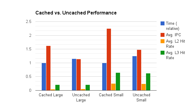
| Run | Time (s) | Avg. IPC | Avg. L2 Hit Rate | Avg. L3 Hit Rate |
|---|---|---|---|---|
| Cached Large | 78.875 | 1.621 | 0.042 | 0.213 |
| Uncached Large | 91.151 | 1.144 | 0.058 | 0.205 |
| Cached Small | 57.243 | 2.245 | 0.257 | 0.642 |
| Uncached Small | 71.422 | 1.485 | 0.242 | 0.624 |
The z-cache increaced performance by 16% for the large runs and 25% for the small! These time improvements are reflected in the average IPC figures. The L2 and L3 cache hit rates remain mostly unchanged, but this makes sense; z-cache or not, the program still needs to hit the grid the same number of times. Unfortunately, PCM doesn't report memory bandwidth on non-Xeon processors and doesn't tell L1 hit rates at all. I'd be interested to see how much work the L1 caches did to increase the IPC so much.
Just for fun, I graphed the IPC and hit rates over time, then overlaid it with the generated fractal and the results are beautiful:
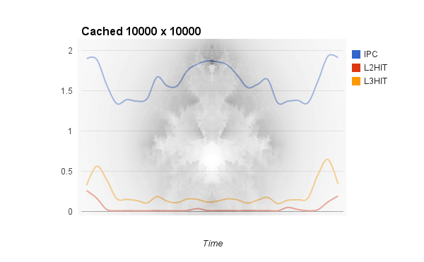
You can see that IPC and L3 hit rates are high where the program processed points that left the Mandelbrot set immediately, while points that stayed in the set longer and caused more grid accesses were correlated with lower IPC and cache rates as the main memory had to be accessed more often. Note that the columns near the left and right sides are processed much more quickly than the ones in the middle, so the graph isn't even overlaid perfectly.
I did the same with the 700 x 700 run, but those results weren't as pretty:
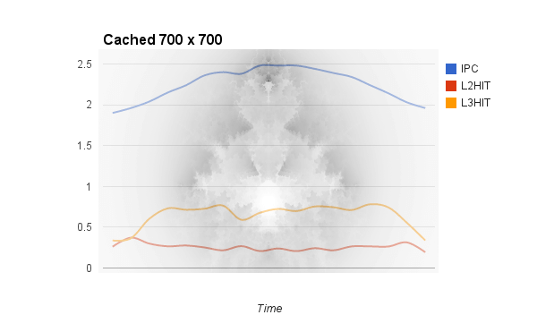
Since the entire working set more or less fits in cache, metrics stayed relatively high throughout the run. IPC seems to follow a bell curve of sorts, mostly immune to the fluctuations seen in the 10k run. I think this is because the more computationally demanding points require more floating point performance and aren't slowed down by system RAM access time anymore, allowing Haswell's full computational power to show through. If you're interested in the other metrics PCM captures, the full data is available here.
That's all I've got for now. If I can think of something I can investigate in the OpenCL code I will some other time.
- Tests performed on an Intel Core i5-4460 with 8 GB DDR3-1866 and an EVGA GeForce GTX 970 with 347.52 drivers on Windows 8.1 Pro x64.↩
- Via SiSoftware↩