Diagram of the feature detection portion of the algorithm

Machine learning is extremely useful in daily life -- Google uses it to fight spam, Facebook uses it to automatically tag your friends in pictures you upload, and many scanners use it to identify handwritten letters in documents to be automatically converted to searchable text. It also requires a huge amount of computation. Input sizes of hundreds of thousands of samples are commonplace, and to fully analyze even small samples can take a long time.

This past semester I took ECE408: Applied Parallel Programming, a class which covered GPGPU computing, specifically CUDA. The final project was very open-ended: we could do whatever we wanted, as long as it used the GPGPU concepts we discussed in class. My group and I looked into some machine learning applications and decided that one, specifically the training phase of object recognition in images using Haar-like classifiers, was both embarrassingly parallelizable and easy to find a large, preformatted training set for. So we planned out our approach and got coding.

The Algorithm

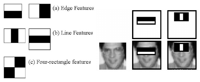Illustration of Haar-like features from OpenCV

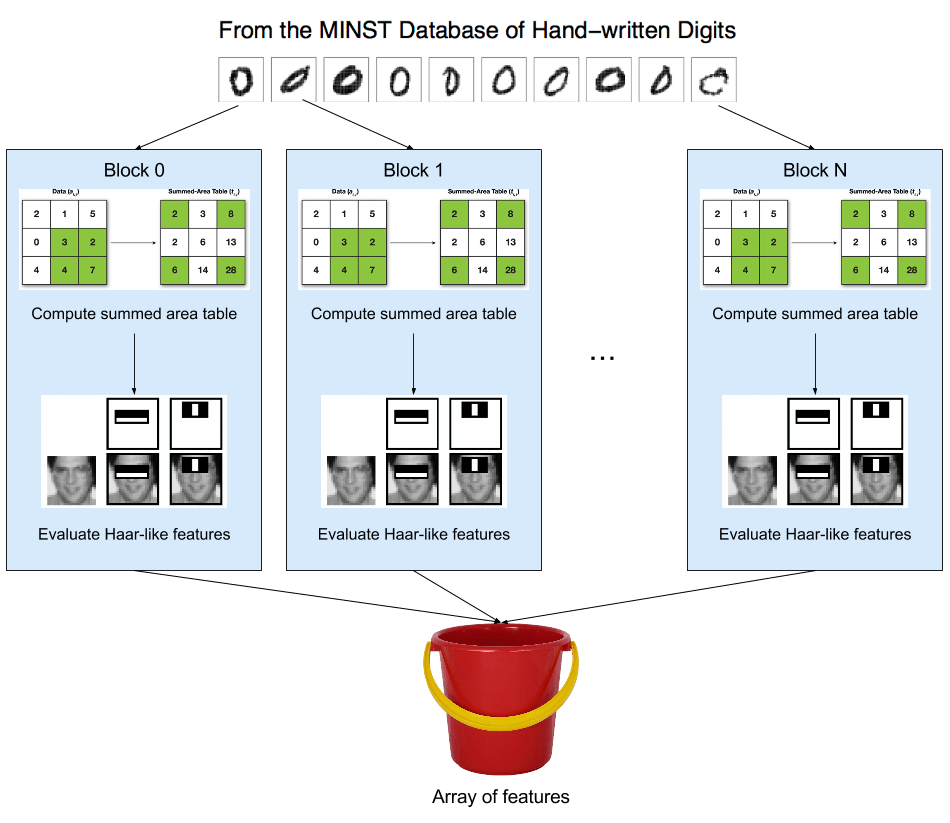
First, a quick overview on how the whole thing works. Our input data set is a large set of images of handwritten digits. The first phase of the training algorithm is to scan each image for Haar-like features. Pictured above, Haar-like features are rectangular blocks containing 50% white regions and 50% black. The algorithm moves and resizes these over every part of each training image, subtracting the intensities of all the pixels in the white region from those of the black region. If the difference is above a set threshold, the location and difference are saved for the next phase.

These individual features are considered weak classifiers because they're unable to positively identify any objects. In fact, they're only slightly better than chance. But when we identify enough of them, determine which are the best, and group them together into a strong classifier, we'll be able to use it to identify objects with a high degree of certainty.

Which brings us to the next phase, AdaBoost. Each feature identified in the previous phase is applied to every image in the training set. If a feature correctly identifies the image, its weight is increased; if it fails to identify the image, its weight is decreased. Images which are correctly identified by lots of features lose weight, causing weak classifiers that correctly identify them to gain less weight than those which identify a more difficult-to-identify image. After a large number of rounds of this, the best features will have the highest weight. We take these features, group them together into a strong classifier, then output them to the object recognition phase.

Parallelization

As I previously mentioned, this process is embarrassingly parallel. Each image can be scanned for features independently of all other images, and each feature on each image can be evaluated independently of all other features on that image. The AdaBoost phase similarly allows each feature to be evaluated on each image independently of all other features and images. Since the input sizes involved are so large (60,000 images, 450,000 features per image, ~70,000,000 features above threshold), massively parallel processors like GPUs fit the problem perfectly. I programmed the feature identifying phase while a group member wrote the AdaBoost section, so the rest of this post will focus on the former.

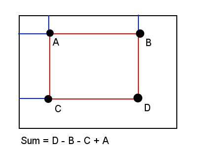Illustration of summed area tables from Wikipedia

Identifying features requires summing up all the pixel values in rectangular regions of the image, an O(nm) operation on the size of the region (n, m). However, there exists a method called integral images, or summed area tables, wherein the sum in a rectangular region of the image can be computed with just four memory reads in constant time. The value of each coordinate (x, y) in the integral image is equal to the sum of all pixels (i, j) with i and j less than or equal to x and y, respectively. I generate this data using a number of parallel prefix scans, first across the rows, then down the columns. Each scan can be done in parallel with just O(logn) steps (where n is the size of the row or column) for each of the 2n rows and columns, for a final parallelized time complexity of O(nlogn).

With that calculation out of the way, the thread block can get to evaluating features. Our images are all 28x28 pixels and the smallest feature size I evaluate is 4x4, giving a total of 90,000 rectangular regions per image. The threads all choose one of these regions and evaluate all five Haar-like features there, save any features that have magnitudes above the predetermined threshold to a buffer shared between all blocks on the grid, then choose another region until there are none left. Thanks to the integral image, each feature can be evaluated in constant time, and since there are O(n⁴) rectangluar regions in an n x n image, each image is analyzed in O(n⁴) time. But thanks to the massive parallelization achievable, even this high-complexity problem can be solved quickly in practice.

Implementation

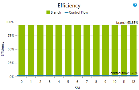Branch efficiency graph for the feature identification phase. Note the low control flow efficiency.

Early on in development, I designed the kernel so that even in the worst case, where every image analyzed contained all 450,000 possible features above the threshold, the output buffer would not overflow. However, since this meant reserving 5.4 MB of global memory per image, the number of images I could analyze per kernel launch was low.

I also had no way to keep track of how much of the buffer actually got used, so I had to copy the whole buffer (around 3 GB) back to the host after each kernel. This transfer took a very long time compared to the computation, so I looked into using CUDA streams to overlap the computation and device-to-host transfers. Unfortunately, CUDA asynchronous transfers require the host buffer to be allocated using pinned memory. But as my computer only had 8 GB of system RAM, allocating 6 GB of it as pinned memory for the two CUDA streams was out of the question.

With streams not a viable option, I instead tried to use bitpacking to reduce the amount of memory each feature consumed, then transfered the packed features to the host and unpacked them using OpenMP. While this approach did reduce the amount of memory used for each image by ⅓, the unpacking process took much longer than the computation and transfer combined, leading to a net slowdown. I shelved the problem, went back to the old implementation, then worked for a day or two on other tasks.

Once I finished the feature magnitude computing code, I revisited the problem. Analyzing the training set with a sufficiently high threshold revealed that on average, each image only had around 1200 useful features. However, some complex images had many times more. After a groupmate realized that the AdaBoost phase did not require the features to be grouped by which images they were found in, I decided that instead of giving each image its own small output buffer, I could give the entire grid one large buffer to share; this way, I didn't have to worry about one or two images with lots of significant features overflowing their buffers. Thanks to the optimized atomic operations in Maxwell, this approach carried virtually no performance penalty. It also allowed me to copy exactly as many features as there were in the buffer directly to the host buffer in one cudaMemcpy call, rather than copy each image's buffer individually. Coupled with the much lower feature count per image compared to my worst-case assumptions, I was able to analyze all the images with just three kernel launches and cudaMemcpy calls rather than the ~200 I originally needed. This completely solved the communications bottleneck.

With the code optimized as I could get it in the time I had, I ran the Nsight performance analyzer to see how much performance I was squeezing out of the card. I saw two problems immediately: control divergence and occupancy.

The control divergence is inherent to this sort of algorithm. While some other algorithms can be optimized ahead of time to minimize the amount of control divergence in each warp, whether or not each thread takes a branch is completely dependent on the input image. As a result, this divergence is inevitable. Nsight reported a control flow efficiency of just 1.76%.

Occupancy, too, was mostly out of my hands. NVCC used over 120 registers per thread, severely limiting the number of active warps on each SM. I could limit the thread count to 64 using a compiler flag, but this caused a drastic decrease in performance. Short of manually writing a PTX version of my code, there wasn't much I could do here.

Despite these issues, my GTX 970 was able to process all 60,000 images in just 9.9 seconds, a 15.3x speedup over the OpenMP implementation running on my i5-4460 and 58.6x faster than the single-threaded code.

Conclusion

Looking back, this ended up being an excellent choice of final project. Machine learning is a very practical field of computer science, and one that I'd never been formally exposed to before. It also fit very well to the CUDA programming model, making it good practice for the material we'd learned all semester. And finally, being able to get a 15.3x speedup over optimized OpenMP code just puts a smile on my face.

The code is available here!